Tech Trend Co-Occurrence Analysis: Mapping the Technology Landscape from 244 Job Postings
How I used Databricks to turn unstructured job descriptions into a network graph of technology ecosystems — with AI extraction, association rule mining, and Louvain community detection.
The Dataset
I started with 244 job descriptions from the data engineering, analytics, and AI space. Each posting had already been processed through Databricks’ ai_extract function, which parsed the unstructured text into structured fields: frameworks, programming languages, and tools/platforms.
The result was a Spark table (workspace.default.jd_tech_extracted) where each job had a clean nested JSON payload of extracted technologies — ready for quantitative analysis.
1. From Nested JSON to a Binary Occurrence Matrix
The ai_extract output stored technologies in three separate arrays (frameworks, programming_languages, tools_and_platforms). The first step was to aggregate them into a single keyword list per posting:
df_keywords = df.selectExpr(
    "path", "file_id",
    """
    filter(flatten(array(
      transform(cast(extracted:response.frameworks
                as array<variant>), x -> cast(x:name.value as string)),
      transform(cast(extracted:response.programming_languages
                as array<variant>), x -> cast(x:name.value as string)),
      transform(cast(extracted:response.tools_and_platforms
                as array<variant>), x -> cast(x:name.value as string))
    )), x -> x is not null) as all_keywords
    """
)
From there, I exploded the keyword arrays to build a sparse binary occurrence matrix X in long form — one row per (file_id, keyword) pair:
df_occurrence = (
    df_keywords
    .select("file_id", explode("all_keywords").alias("keyword"))
    .filter(col("keyword").isNotNull() & (col("keyword") != ""))
    .distinct()
)
n_postings = df_keywords.count()    # 244
n_tech = df_occurrence.select("keyword").distinct().count()  # 617
# Total mentions: 1,805
617 unique technologies across 244 postings, with 1,805 total mentions. The most frequently requested technologies:
- SQL: 113 postings (46%)
- Python: 98 postings (40%)
- Power BI: 78 postings (32%)
- AWS: 47 postings (19%)
- Databricks: 46 postings (19%)
- Azure: 40 postings (16%)
SQL and Python dominate, appearing in nearly half of all job descriptions. But raw frequency alone doesn’t tell us which technologies form real ecosystems.
2. Computing the Co-Occurrence Matrix
To find which technologies appear together, I computed the co-occurrence matrix C = Xᵀ × X by self-joining the occurrence table on file_id:
df_cooccur = (
    df_occurrence.alias("a")
    .join(df_occurrence.alias("b"), on="file_id", how="inner")
    .select(col("a.keyword").alias("keyword_a"),
            col("b.keyword").alias("keyword_b"))
    .groupBy("keyword_a", "keyword_b")
    .agg(count("*").alias("cooccur_count"))
)
This produced 16,801 unique (keyword_a, keyword_b) pairs — every combination of technologies that appeared together in at least one posting.
The top raw co-occurrences:
- SQL ↔ Power BI: 62 postings
- Python ↔ SQL: 58 postings
- Power BI ↔ Python: 34 postings
- Databricks ↔ SQL: 33 postings
- SQL ↔ Azure: 29 postings
- AWS ↔ Python: 26 postings
Not surprising — these are the most frequent technologies individually. The real signal is in which pairs co-occur far more than their individual frequencies would predict.
3. Association Metrics: Phi, Lift, and Confidence
For every pair of technologies (A, B), I built a 2×2 contingency table:
# Contingency table for pair (A, B):
# |             | B present | B absent | Total |
# | A present   | n11       | n10      | n1x   |
# | A absent    | n01       | n00      | n0x   |
# | Total       | nx1       | nx0      | N     |
Here’s a concrete example: Databricks × Azure
2×2 Contingency Table: Databricks × Azure  (n = 244)

                          Azure=1      Azure=0        Total
──────────────────────────────────────────────────────────
Databricks=1                   18           28           46
Databricks=0                   22          176          198
──────────────────────────────────────────────────────────
Total                          40          204          244

Under H₀ (independence), expected n₁₁ = 46 × 40 / 244 = 7.54
Observed n₁₁ = 18 → Lift = 2.387
Databricks and Azure co-occur 2.4× more often than random chance would predict. That’s a meaningful association — not just two popular technologies being popular.
I computed three metrics for every pair in a single Spark pipeline:
df_stats = df_pairs
    .join(df_diag.alias("da"), ...)
    .join(df_diag.alias("db"), ...)
    .withColumn("phi",
        (col("n11") * col("n00") - col("n10") * col("n01")) /
        sqrt(col("n_a") * (N - col("n_a")) *
             col("n_b") * (N - col("n_b")))
    )
    .withColumn("lift",
        (col("n11") * N) / (col("n_a") * col("n_b"))
    )
    .withColumn("confidence",
        col("n11") / col("n_a")
    )
4. Filtering for Signal
To cut through the noise, I applied three thresholds before building the network:
- Minimum co-occurrence (n11 ≥ 3) — avoid one-off pairs
- Minimum lift > 1.5 — co-occur at least 50% more than chance
- Both technologies appear in at least 3 postings — exclude rare techs
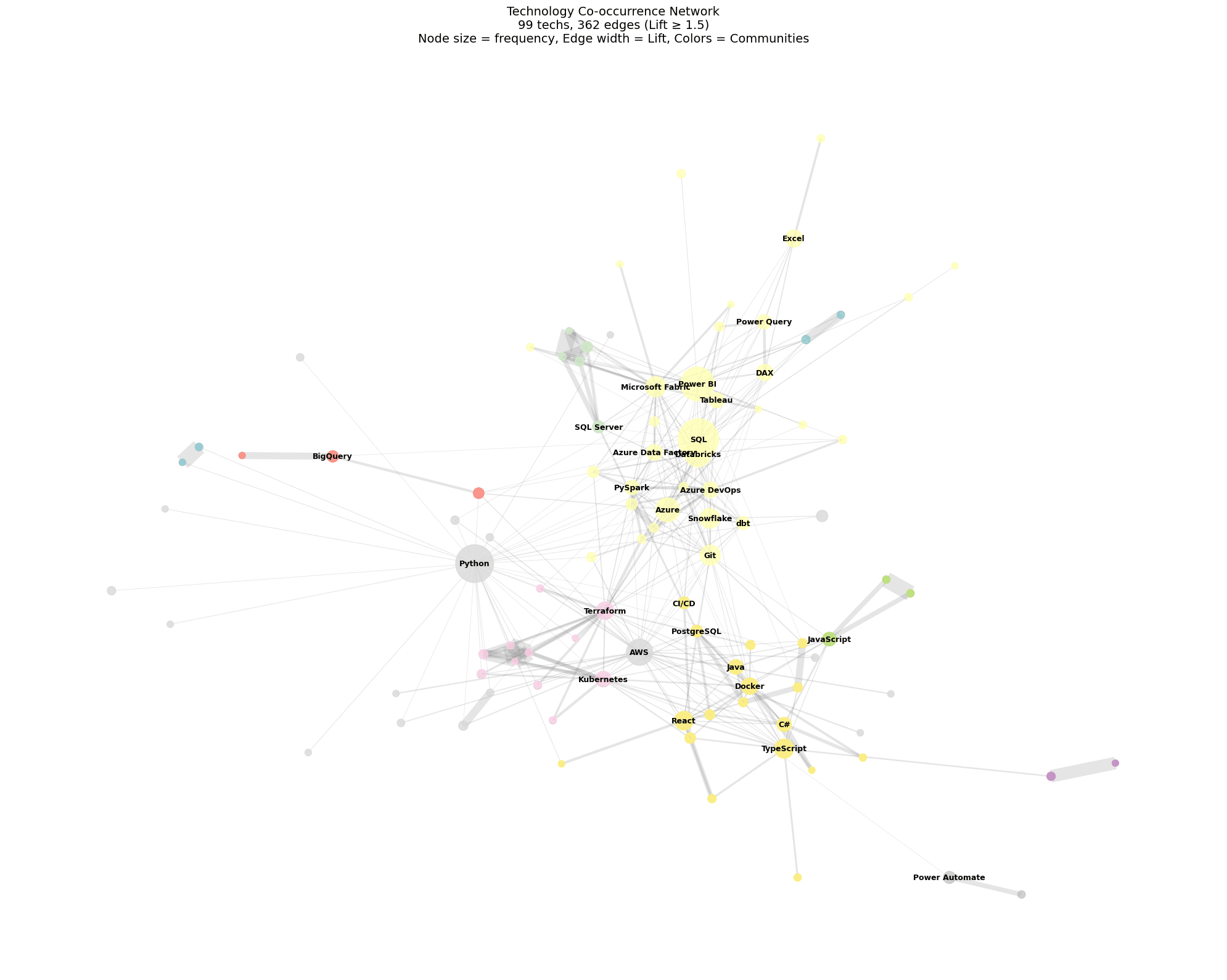
This reduced the 16,801 raw pairs down to 362 statistically meaningful edges connecting 99 technologies in the largest connected component.
Some of the strongest associations:
Microsoft DevOps ↔ SSRS: n11=3, Lift=40.7, φ=0.70 — a tightly coupled Microsoft BI toolchain
SQL Server ↔ SSAS: n11=3, Lift=18.3, φ=0.46 — classic Microsoft data warehousing stack
CI/CD pipelines ↔ Kubernetes: n11=3, Lift=6.2, φ=0.24 — DevOps infrastructure pairing
Azure ↔ PySpark: n11=6, Lift=2.6, φ=0.18 — cloud + big data processing
Databricks ↔ SQL: n11=33, Lift=1.55, φ=0.25 — high co-occurrence, moderate lift (both are independently popular)
5. Network Graph & Community Detection
I built an undirected graph with NetworkX — nodes sized by frequency, edges weighted by lift, and communities detected using the Louvain algorithm (which maximizes modularity to find natural clusters):
G = nx.Graph()
for _, row in nodes.iterrows():
    G.add_node(row["tech"], freq=row["freq"])
for _, row in edges.iterrows():
    G.add_edge(row["tech_a"], row["tech_b"],
               weight=row["lift"], n11=row["n11"], phi=row["phi"])

# Louvain community detection
communities = community_louvain.best_partition(G_main, weight="weight")
The algorithm detected 11 distinct technology communities — each mapping to a real-world engineering ecosystem:
- Community 1 — Microsoft/Azure Ecosystem (33 techs): SQL, Power BI, Databricks, Azure, Microsoft Fabric — the dominant cluster. Azure-adjacent data engineering and analytics roles.
- Community 2 — AWS/Data Science Stack (18 techs): Python, AWS, R, Lambda, GitHub — cloud-native data science with AWS’s toolchain.
- Community 3 — Full-Stack Engineering (18 techs): TypeScript, React, Docker, Java, C# — traditional software engineering roles requiring both frontend and backend skills.
- Community 4 — DevOps & Cloud Native (11 techs): Terraform, Kubernetes, GitHub Actions, Go, IAM — infrastructure-as-code and container orchestration.
- Community 5 — Microsoft BI/DWH (5 techs): SQL Server, SSIS, SSRS, SSAS, Microsoft DevOps — the classic on-premise Microsoft BI stack, still very much in demand.
- Community 6 — GCP Ecosystem (3 techs): BigQuery, GCP, Cloud Composer — a small but tight cluster of Google Cloud Platform technologies.
- Community 7 — AI Agents (2 techs): LangGraph, CrewAI — emerging AI agent frameworks forming their own niche.
- Community 8 — AI Coding Assistants (2 techs): Claude Code, Codex — AI coding tools appearing together in forward-looking roles.
- Community 9 — Lakehouse Architecture (2 techs): Lakehouse, Dataflows — the modern data architecture pattern.
- Community 10 — Automation (2 techs): Power Automate, Copilot — low-code automation and AI assistant pairing.
6. Interactive Visualization
I exported the graph to an interactive Plotly HTML file saved to the Databricks Workspace, with hover tooltips showing each technology’s frequency, community, degree, and top connections.
Key Takeaways
- The Microsoft/Azure ecosystem is the largest cluster (33 technologies) — reflecting the dataset’s data engineering and analytics focus.
- AI agent frameworks (LangGraph, CrewAI) and AI coding tools (Claude Code, Codex) already form distinct clusters — these are emerging specializations, not just buzzwords.
- Lift reveals what raw counts hide. SQL–Power BI has high co-occurrence (62), but only moderate lift because both are independently popular. CI/CD pipelines–Kubernetes (n11=3) has lift > 6 — a genuinely tight architectural pairing.
- The GCP ecosystem is small but tight — BigQuery, GCP, and Cloud Composer form a cohesive cluster with high internal lift.
- 519 of 617 technologies had no strong connections after filtering — most listed technologies are isolated mentions, not part of a recognizable stack.